3. Web Services
This chapter describes how OGC OWS web services are realized on top of the converted/transformed data as described in the data chapter. In particular:
- WFS and WMS-Time services
- OWS SOS service
3.1. Architecture
Figure 1 sketches the overall SOSPilot architecture with emphasis on the flow of data (arrows). Circles depict harvesting/ETL processes. Server-instances are in rectangles. Datastores the “DB”-icons.
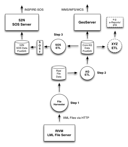
Figure 1 - Overall Architecture
3.2. WFS and WMS Services
This describes the realization of WFS and WMS(-Time) in GeoServer.
GeoServer can directly generate OWS services from a Postgres/PostGIS datasource as one Layer per Table (or View).
For our purpose the source tables are the
stations table and measurements tables in the Postgres schema rivm-lml.
See the data chapter for info how these tables are continuously populated from the raw AQ data via
ETL Step 1 and Step 2.
3.2.1. Database VIEWs
As WFS and WMS always need a geometry-column, we will JOIN
the stations table and the measurements tables to create ‘Postgres VIEWs’.
A VIEW is basically a query but presented as a database table. Data in the VIEW is always current with the original tables
(or VIEWs, as we may derive VIEWs from VIEWs). This way data selections can be provided permanently
and tailored to the particular OWS service.
Having all data (stations, measurements) stored PostgreSQL tables gives rise to many possibilities
for selection from these two tables. The stations table looks as follows.
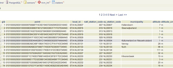
Figure - RIVM Eionet Stations Read into Postgres/PostGIS
The sample-data is stored in the measurements table, as below. station_id is a foreign key
(though not strictly, as new stations may pop-up) into the stations table.
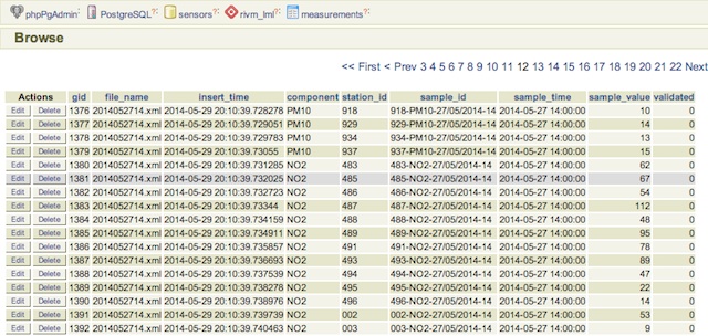
Figure - LML raw measurements stored in Postgres
One appearent VIEW is to combine the measurements and stations tables into a new measurements_stations
table by means of a JOIN query as follows (rivm_lml is the schema name):
CREATE VIEW rivm_lml.measurements_stations AS
  SELECT m.gid, m.station_id, s.municipality, m.component, m.sample_time, m.sample_value, s.point, m.validated,
         m.file_name, m.insert_time, m.sample_id,
         s.local_id, s.eu_station_code, s.altitude, s.area_classification,
         s.activity_begin, s.activity_end
         FROM rivm_lml.measurements as m
           INNER JOIN rivm_lml.stations as s ON m.station_id = s.natl_station_code;
The data can now be viewed as rows in the measurements_stations VIEW, where each sample also has a POINT-geometry:
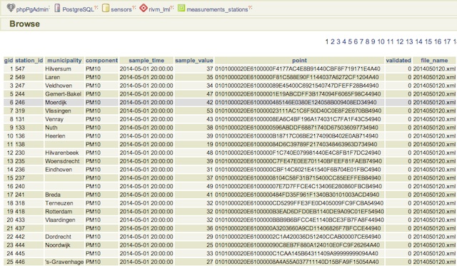
Figure - LML Postgres VIEW of combined measurements and stations
Still this VIEW is too broad to use for WMS/WFS Layers as we will usually visualize (via WMS) or query (via WFS)
a single chemical component. We will use the measurements-stations VIEW to derive more specialized,
per-component VIEWs Two broad VIEWs are provided first:
- per component last-captured measurements
- per component time-series measurements
These VIEWs are in SQL as below taking two components (NO2 and O3) as example.
-- per component last-captured measurements
CREATE VIEW rivm_lml.v_last_measurements_NO2 AS
  SELECT DISTINCT ON (station_id) station_id,
    municipality, sample_time, sample_value, point, validated, gid, sample_id
  FROM rivm_lml.measurements_stations WHERE component = 'NO2' ORDER BY station_id, gid DESC;

CREATE VIEW rivm_lml.v_last_measurements_O3 AS
  SELECT DISTINCT ON (station_id) station_id,
    municipality, sample_time, sample_value, point, validated, gid, sample_id
  FROM rivm_lml.measurements_stations WHERE component = 'O3' ORDER BY station_id, gid DESC;

 .
 .

-- per component time-series measurements
CREATE VIEW rivm_lml.v_measurements_NO2 AS
  SELECT  station_id,
    municipality, sample_time, sample_value, point, validated, gid, sample_id
  FROM rivm_lml.measurements_stations WHERE component = 'NO2';

CREATE VIEW rivm_lml.v_measurements_O3 AS
  SELECT  station_id,
    municipality, sample_time, sample_value, point, validated, gid, sample_id
  FROM rivm_lml.measurements_stations WHERE component = 'O3';
  .
  .
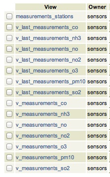
Figure - All database views
Data from these VIEWs can now be viewed as rows like in this table:
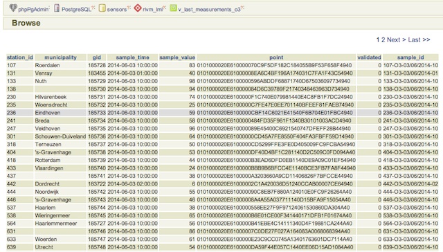
Figure - LML Postgres VIEW of last measured values at each station for Ozone
3.2.1.1. Additional VIEWs
Additional VIEWs for the future can be thought, like:
- averages
- peak values
- even Voronoi-data can be derived, though that may be expensive: http://smathermather.wordpress.com/2013/12/21/voronoi-in-postgis
These VIEWs can readily applied for WMS with legenda’s like here: http://www.eea.europa.eu/data-and-maps/figures/rural-concentration-map-of-the-ozone-indicator-aot40-for-crops-year-3
3.2.1.2. GeoServer Service Creation
From the above database VIEWs the WMS/WFS Layers can be created in the GeoServer Admin GUI. The main items to develop specifically are the Styled Layer Descriptors (SLDs). The choice is to provide colouring schemes for ranges of values or just labels showing the values. The latter has been chosen initially.
The challenge is to do something interesting with the Time aspect (field sample_time) as
all features would be positions at the same (station) point coordinates.
For WMS we can use WMS-Time, for WFS we may provide search forms with queries. Other visualizations may be interesting like Voronoi diagrams: http://smathermather.wordpress.com/2013/12/21/voronoi-in-postgis/.
All OWS services are available from this URL: http://sensors.geonovum.nl/gs/sensors/ows
The WFS capabilities: http://sensors.geonovum.nl/gs/wfs?request=GetCapabilities
The WMS Capabilities: http://sensors.geonovum.nl/gs/wms?request=GetCapabilities
Within the GeoServer Admin GUI, a PostGIS datastore is added, with the schema rivm-lml.
From there on various wizards and forms will lead to Layer creation and configuration.
3.2.2. WMS TIME Dimension
The OGC has defined additional WMS 1.3 practises for working with Dimensions, and in particular with Time and Elevation: https://portal.opengeospatial.org/files/?artifact_id=56394
GeoServer supports these extensions via a ‘Dimensions’ tab in each Layer configuration.
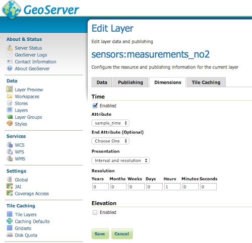
Figure - WMS Configuration for Time Dimension
The sample_time date-field is selected, the data is presented as `Interval and resolution’ with a resolution
of 1 hour as this is the standard interval for LML measurements.
The Capabilities also show for the <component>_measurements Layers the Time dimension.
See figure below.
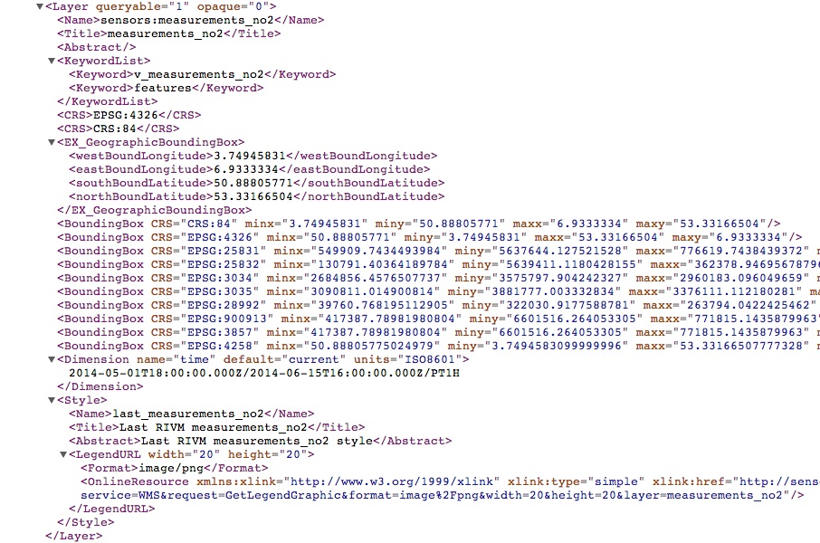
Figure - WMS Capabilities Layer with Time Dimension
3.2.3. Stations Layer
This is quite trivial: a small flat table with station info and a Point geometry. The WMS layer may be added to a viewer like the KadViewer: http://kadviewer.kademo.nl or any other GIS package.
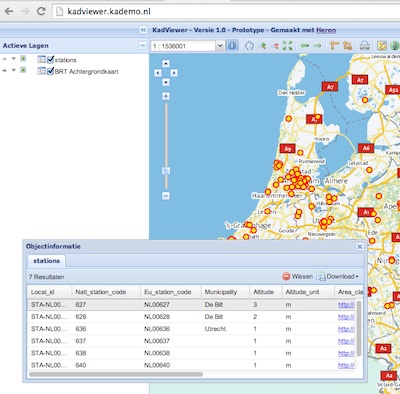
Figure - GeoServer stations WMS Layer with FeatureInfo
3.2.4. Measurements Layers
These layers are created from the individual per-component VIEWs described above.
For each component there are last_measurements_<component> and a measurements_<component> Layers.
3.2.5. Styled Layer Descriptors
A simplified SLD approach is taken, just circles with a text label for values. More advanced
SLDs may be added later. Here is an example for NO2, both used for the measurements_no2 and last_measurements_no2
layers.
<?xml version="1.0" encoding="ISO-8859-1"?>
<StyledLayerDescriptor version="1.0.0"
                       xsi:schemaLocation="http://www.opengis.net/sld StyledLayerDescriptor.xsd"
                       xmlns="http://www.opengis.net/sld"
                       xmlns:ogc="http://www.opengis.net/ogc"
                       xmlns:xlink="http://www.w3.org/1999/xlink"
                       xmlns:xsi="http://www.w3.org/2001/XMLSchema-instance">

    <!-- a Named Layer is the basic building block of an SLD document -->
    <NamedLayer>
        <Name>last_measurements_no2</Name>
        <UserStyle>
            <!-- Styles can have names, titles and abstracts -->
            <Title>Last RIVM measurements_no2</Title>
            <Abstract>Last RIVM measurements_no2 style</Abstract>
            <IsDefault>1</IsDefault>
            <!-- FeatureTypeStyles describe how to render different features -->
            <!-- A FeatureTypeStyle for rendering points -->
            <FeatureTypeStyle>
                <Rule>
                    <PointSymbolizer>
                        <Graphic>
                            <Mark>
                                <WellKnownName>circle</WellKnownName>
                                <Fill>
                                    <CssParameter name="fill">#8b008b</CssParameter>
                                    <CssParameter name="fill-opacity">1.0</CssParameter>
                                </Fill>
                                <Stroke>
                                    <CssParameter name="stroke">#ee82ee</CssParameter>
                                    <CssParameter name="stroke-width">1</CssParameter>
                                </Stroke>
                            </Mark>
                            <Size>30</Size>
                        </Graphic>
                    </PointSymbolizer>

                    <TextSymbolizer>
                        <Label>
                            <ogc:PropertyName>sample_value</ogc:PropertyName>
                        </Label>
                        <Font>
                            <CssParameter name="font-family">
                                <ogc:Literal>Lucida Sans Regular</ogc:Literal>
                            </CssParameter>

                            <CssParameter name="font-size">
                                <ogc:Literal>10</ogc:Literal>
                            </CssParameter>
                            <CssParameter name="font-weight">
                                <ogc:Literal>bold</ogc:Literal>
                            </CssParameter>
                        </Font>
                        <LabelPlacement>
                            <PointPlacement>
                                <AnchorPoint>
                                    <AnchorPointX>0.5</AnchorPointX>
                                    <AnchorPointY>0.5</AnchorPointY>
                                </AnchorPoint>
                            </PointPlacement>
                        </LabelPlacement>
                        <Fill>
                            <CssParameter name="fill">#ffffff</CssParameter>
                        </Fill>
                    </TextSymbolizer>
                </Rule>
            </FeatureTypeStyle>
        </UserStyle>
    </NamedLayer>
</StyledLayerDescriptor>
These layers can be rendered in any WMS viewer, but in particular viewers that support the WMS-Time parameter on the client, for example the HeronViewer developed for this project. Heron is a web mapping client framework that builds on OpenLayers . OL supports WMS Dimensions in general.
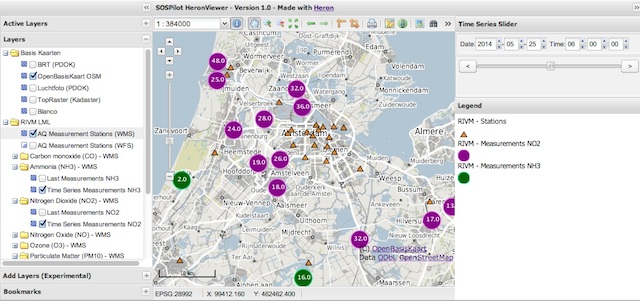
Figure - Heron Viewer showing WMS-T Measurements Layers
3.2.6. WFS Layers
WFS Layers are created automatically for each WMS Layer in GeoServer. A WFS query can be as follows:
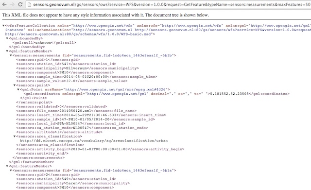
Figure - GeoServer measurements Layer WFS query
3.3. SOS Services
“The OGC Sensor Observation Service aggregates readings from live, in-situ and remote sensors. The service provides an interface to make sensors and sensor data archives accessible via an interoperable web based interface.”
The chapter on server administration describes how the 52 North SOS server is deployed. This is called here the ‘SOS Server’.
Different as from GeoServer the ‘SOS Server’ comes with its own database schema and store. Via ETL Step 3 as described in the data chapter, the tables are populated by publishing both sensor and observation data via SOS-Transactions to the SOS Server. There is no need to, like with GeoServer, to configure SOS services as these are readily available.
A later option is to directly couple the Core AQ tables to the SOS server via a mapping config.
The SOS server is available at this endpoint: http://sensors.geonovum.nl/sos Note that this server also supports the REST API as specified in: http://sensorweb.demo.52north.org/sensorwebclient-webapp-stable/api-doc/index.html. The REST API is at: http://sensors.geonovum.nl/sos/api/v1/
On June 13, 2014, a first test was performed integrating Air Quality SOSs from Belgium, Holland and Sweden via the 52 North HTML5 client. This gave a promising result as depicted below.
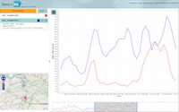
Figure - GeoServer measurements Layer WFS query
From: Simon Jirka ....... during the last days, the SOS servers form the Netherlands and also from Sweden went online. We have used this opportunity to connect our client to all three servers and to load Ozone data. Attached you find a screenshot of the result. The data from Sweden is coloured in green, the time series from Belgium is blue and the data from the Netherlands has red colour. Data from the SOS operated by the EEA should follow next week, as well.