7. Applying RIO for AQ Data
Starting in october 2015 the SOSPilot platform was extended to handle Air Quality data using the RIO model.
RIO is an interpolation method/tool for Air Quality data. Get a global overview from the IrCELine website and the article “Spatial interpolation of air pollution measurements using CORINE land cover data” for scientific details.
The RIO tools are used by RIVM, see the RIVM website:
“Het RIVM presenteert elk uur de actuele luchtkwaliteitskaarten voor stikstofdioxide, ozon en fijn stof in Nederland op de website van het Landelijk Meetnet Luchtkwaliteit (LML). Meetgegevens van representatieve LML-locaties worden gebruikt om te berekenen wat de concentraties voor de rest van Nederland, buiten de meetpunten om, zijn. De huidige rekenmethode om deze kaarten te maken, genaamd INTERPOL, heeft een aantal beperkingen. Hierdoor worden bijvoorbeeld stikstofdioxideconcentraties in stedelijk gebied vaak onderschat.
In België is een betere interpolatiemethode ontwikkeld. Deze methode, de RIO (residual interpolation optimised for ozone) interpolatiemethode, wordt daar gebruikt voor luchtkwaliteitskaarten die het publiek informeren over de actuele luchtkwaliteit. In 2009 is de RIO interpolatiemethode in opdracht van het RIVM zodanig uitgebreid en aangepast dat hij ook in Nederland kan worden gebruikt.”
A RIO toolkit, has been developed by VITO, a leading European independent research and technology organisation based in Belgium. The toolkit is implemented in MatLab. Basically the RIO-tool converts Air Quality measurement data (CSV) from a set of dispersed stations to country-wide (RIO needs to be tailored per country) coverage data. RIVM uses RIO to produce and publish daily maps of Air Quality data for NO2, O3 and PM10, like the image below.
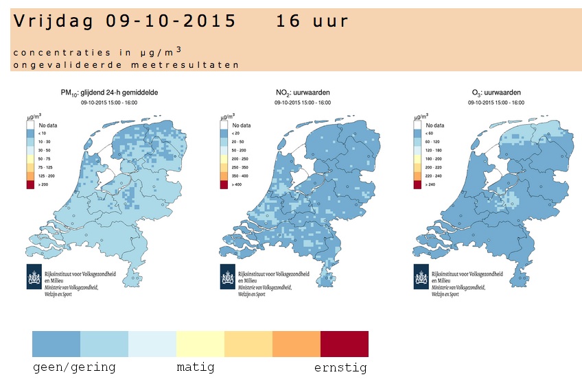
Website www.lml.rivm.nl - dispersion maps produced with Rio
7.1. The Plan
The plan within the SOSPilot project is as follows:
- apply the RIO model/tool to crowd-sourced air quality measurements, in particular from the Smart Emission Project Project
- unlock RIO output via an OGC Web Coverage Service (WCS)
Once the above setup is working, various use-cases will be established, for example combining AQ coverage data with other INSPIRE themes like population and Netherlands-Belgium cross-border AQ data dispersion.
WCS is also a protocol for INSPIRE Download Services (together with WFS and SOS). This is also the main reason for the above plan. The RIO model also uses data from other INSPIRE themes, in particular land coverage (CORINE).
See also an overview in this presentation (Grothe 2015) from which the image below was taken.
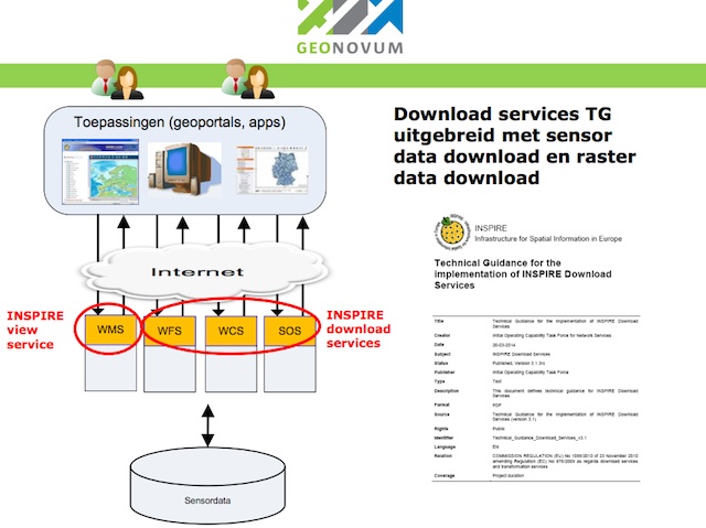
INSPIRE View and Download Services
7.2. RIO Output via WCS
This was done as a first step. RIVM has kindly provided us with some RIO input and output datafiles plus documentation.
These can be found here. The aps2raster directory
contains the resulting GeoTIFF files. The work was performed under this GitHub issue.
7.2.1. APS Files
RIO output files are text-files in the so-called APS format. An APS file starts with a single line of metadata. Its format is described in the APS-header documentation. Subsequent lines are the rows forming a 2-dimensional array with the interpolated values.
Below is an example APS header:
# APS Header
# Y  M  D  H  C   unit  sys   comment  format  proj  orig_x  orig_y  cols rows  pix_w  pix_h
# 15 9 16 10 NO2 ug/m3 RIO  uurwaarden f7.1    1     0.000   620.000 70    80   4.000  4.000
The metadata gives enough information to construct a GeoTIFF. The most important parameters are
- origin X, Y of coverage
- pixel width and height
- date and time (hour) of the measurements
- the chemical component (here NO2)
The data values are space-separated values. Empty (NoData) values are denoted with -999.0 :
... -999.0   23.4   23.6 -999.0   24.2   17.3   14.3 ...
...   16.1   17.3   18.4   19.4   21.6   21.9   20.1 ...
7.2.2. Converting to GeoTIFF
Developing a simple Python program called aps2raster.py,
the .aps files are converted to GeoTIFF files. aps2raster.py reads an APS file line by line. From the first
line the metadata elements are parsed. From the remaining lines a 2-dimensional array of floats is populated.
Finally a GeoTIFF file is created with the data and metadata. Projection is always in RD/EPSG:28992.
aps2raster.py uses the GDAL and NumPy Python libraries.
7.2.3. WMS with Raster Styling
Using GeoServer the GeoTIFFs are added as datasources and one layer per GeoTIFF is published. Within GeoServer this automatically creates both a WCS and a WMS layer. As the GeoTIFF does not contain colors but data values, styling is needed to view the WMS layer. This has been done via Styled Layer Descriptor (SLD) files. GeoServer supports SLDs for Rasterdata styling. In order to render the same colors as the RIVM LML daily images a value-interval color-mapping was developed as in this example for NO2:
<FeatureTypeStyle>
<FeatureTypeName>Feature</FeatureTypeName>
<Rule>
<RasterSymbolizer>
<ColorMap type="intervals">
<ColorMapEntry color="#FFFFFF" quantity="0" label="No Data" opacity="0.0"/>
<ColorMapEntry color="#6699CC" quantity="20" label="< 20 ug/m3" opacity="1.0"/>
<ColorMapEntry color="#99CCCC" quantity="50" label="20-50 ug/m3" opacity="1.0"/>
<ColorMapEntry color="#CCFFFF" quantity="200" label="50-200 ug/m3" opacity="1.0"/>
<ColorMapEntry color="#FFFFCC" quantity="250" label="200-250 ug/m3" opacity="1.0"/> <!-- Yellow -->
<ColorMapEntry color="#FFCC66" quantity="350" label="250-350 ug/m3" opacity="1.0"/>
<ColorMapEntry color="#FF9966" quantity="400" label="350-400 ug/m3" opacity="1.0"/>
<ColorMapEntry color="#990033" quantity="20000" label="> 400 ug/m3" opacity="1.0"/>
</ColorMap>
</RasterSymbolizer>
</Rule>
</FeatureTypeStyle>
The SLD files can be found here.
The WMS layers have been added to the existing SOSPilot Heron viewer.
7.2.4. Comparing with RIVM LML
The resulting WMS layers can now be compared to the original PNG files that came with the APS data files from RIVM. Below two examples for NO2 and PM10.
For NO2 below.
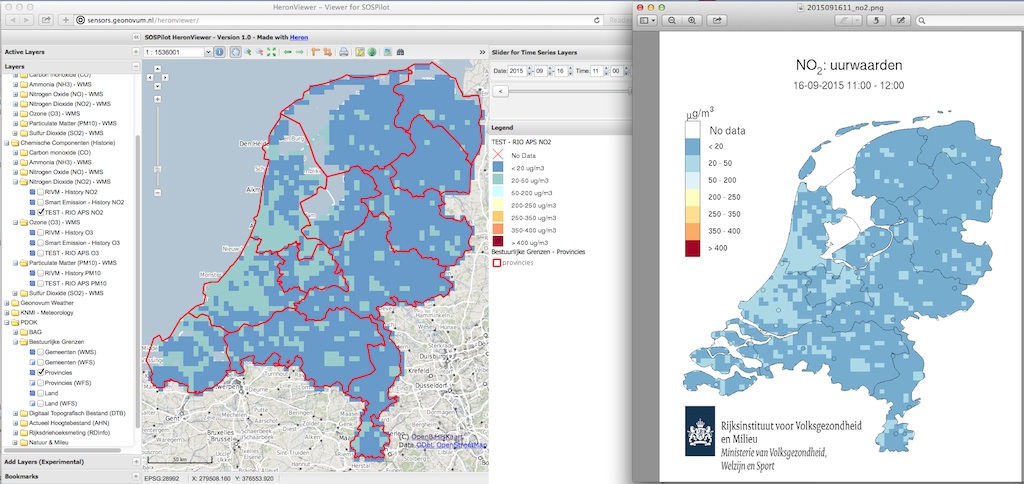
Comparing with RIVM LML maps (right) - NO2
And for PM10 below.
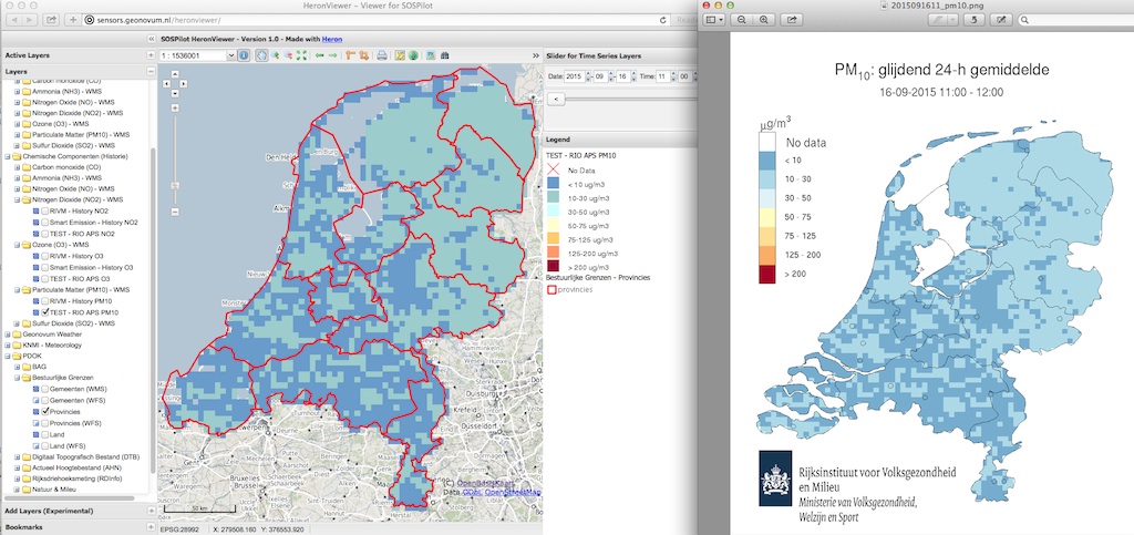
Comparing with RIVM LML maps (right) - PM10
As can be seen the maps are identical. Our WMS-maps are on the left, RIVM maps on the right. Our WMS maps are somewhat “rougher” on the edges since we have not cut-out using the coastlines.
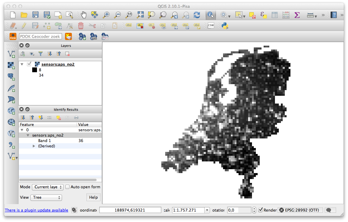
7.2.5. WCS in QGIS
The Layers published in GeoServer can be viewed in QGIS by adding a WCS Layer via the standard WCS support in QGIS.
INSPIRE View and Download Services
7.3. Viewing Results
Results can be viewed in basically 3 four ways:
- as WMS Layers via the Heron Viewer: http://sensors.geonovum.nl/heronviewer
- as WCS in e.q. QGIS http://sensors.geonovum.nl/gs/sensors/wcs?
- via direct WCS protocol requests
- as raw GeoTIFF raster files
Below some guidance for each viewing method. TBS
7.3.1. Heron Viewer
Easiest is to use the predefined map-context bookmarks (see also the tab “Bookmarks” on the left panel):
- NO2 coverage: http://sensors.geonovum.nl/heronviewer/?bookmark=rivmriono2
- O3 coverage: http://sensors.geonovum.nl/heronviewer/?bookmark=rivmriono3
- PM10 coverage: http://sensors.geonovum.nl/heronviewer/?bookmark=rivmriopm10
Or by hand: go to http://sensors.geonovum.nl/heronviewer
- left are all map-layers organized as a collapsible explorer folders
- find the folder named “Chemische Componenten (Historie)”
- open this folder
- open subfolder named “Nitrogen Dioxide (NO2) - WMS”
- activate the map-layer named “TEST RIO APS NO2”
These values can be compared with the WMS-Time Layer-based values for the same component, for example for NO2:
- within the same submap “Nitrogen Dioxide (NO2) - WMS”
- enable the WMS-Time Layer “RIVM History - NO2”
- use the Timeslider in the upper right of the viewer
- slide the date/time to September 16, 2015 11:00
- compare the values by clicking on the circles, a pop-up opens for each click
- you may first want to disable the stations layers
7.3.2. WCS in QGIS
See above. WCS link is http://sensors.geonovum.nl/gs/sensors/wcs?. There are 3 layers.
7.3.3. WCS Protocol Requests
Direct requests to GeoServer, using the WCS 2.0.1 protocol:
- Fetch WCS Capabilities 2.0.1
- Fetch WCS DescribeCoverage 2.0.1
- Fetch WCS GetCoverage, 41kB GeoTIFF
- Fetch WCS GetCoverage, plain text
7.3.4. Raw Coverage Files
Get GeoTIFF Files from raw GeoTIFF raster files. or via WCS GetCoverage, 41kB GeoTIFF.
7.4. Future Enhancements
7.4.1. WCS and WMS as time-series
Traditional WMS-Time layers are based on vector-data, where a single column in the source data denotes time (or any other dimension like elevation). GeoServer also supports time-series for raster data.
Each coverage now is a snapshot for a single chemical component for a single hour on s single date. To unlock multiple coverages as a time-series the GeoServer ImageMosaic with time-series support can be applied, see this link.
Another posibility is a GeoServer plugin for “Earth Observation profile of coverage standard”, see http://docs.geoserver.org/latest/en/user/extensions/wcs20eo/index.html and http://www.opengeospatial.org/standards/requests/81